Building a math model of a 4-way valve

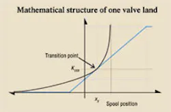
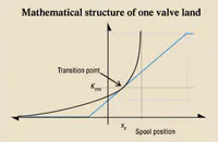
Hydraulicspneumatics Com Sites Hydraulicspneumatics com Files Uploads Custom Inline Archive Www hydraulicspneumatics com Content Site200 Articles 11 01 2011 88191buildingma 00000060762

Figure 1. Modeling of a 4-way valve begins with a single land and two describing equations, one each for the overlap and underlap condition, and intersecting with equal slopes.

A proposed spool valve model is based on the characteristics of a single, variable valve land, four of which are grouped to form the 4-way model. Each land has two regions; the first is the overlap (closed) region in which land-to-land leakage varies in direct proportion to the square root of the differential pressure across the land and is inversely proportional to the overlap distance.

The second region is where the valve land is under lapped and, therefore, is open. This is where the valve coefficient varies in direct proportion to the land under lap (degree of opening) and in direct proportion to the square root of the differential pressure. It is sometimes referred to as the straight line region.

The two regions converge on the transition point, K_VXX in Figure 1. The transition point occurs at a spool position of x_X. The assumption that leakage varies with the square root of pressure drop (it is turbulent) provides the major compromise to achieve mathematical simplicity. And because the valve coefficient varies linearly with land opening, it also points out the applicability only to valves with rectangular metering slots.

Examining the parameters

Figure 2. Land-to-land leakage testing is done with work ports blocked, and each land is assumed to have a flow coefficient of KVXX. This illustration is valid only at the spool position of peak leakage.

Figure 2 is an analytical schematic of the valve when tested for internal leakage and with the spool in the position that results in maximum land-toland leakage. Because it is a symmetrical valve, each land is assumed to have the same value for K_VXX, the flow coefficient at the transition point. The series-parallel configuration can be replaced by a single orifice of K_VTXX , where the addition of the T in the subscript represents total.

K_VTXX is only an estimate of the peak value that will result from the model. At model development time we do not know the transition position of the spool, the intercept value of the open metering land coefficient, nor the scaling coefficient in the overlap region. Also, the exact position of the spool where leakage maximizes is unknown; it is merely estimated from the targeted value of the overlap for the valve’s test data.

An important issue not yet covered is that model development has been done on only one of four individual lands, two of which move toward opening while the other two move toward closure. K_VXX merely corresponds to the transition point; it does not ensure that it will be the point of maximum leakage when all four lands are put together. Therefore, the resulting model will approximate the actual valve test data, but with a complete steady-state performance simulation. A few iterations can be set up to produce the land-to-land leakage in the full bridge circuit and overlap as contained in the actual valve's test data.

It is not uncommon in simulation to start with a perfectly symmetrical valve configuration and then explore various degrees of asymmetry for each of the lands. The proposed valve is a 4-land, 4-way, single spool valve. As such, all lands reside on the same physical spool. As one land moves, all others do too by exactly the same amount. All lands open and close in a synchronized and complementary action to achieve the direction and flow desired.

It’s all in the timing

Figure 3. The timing diagram for each land of our 4-way valve model shows that as the PA and BT lands open from positive spool displacement, the PB and AT lands go into overlap, and vice-versa for negative spool displacement.

As the spool moves, two lands open. One is a powered land, so called because it is in direct communication with the valve's P port. The other is the return land, so named because it is in direct communication with the T port.

At the same time, the other two lands both move into overlap, sometimes erroneously called closure. The exact occurrence in which the four lands open and close is called the valve timing. In a real valve, the only way to alter the valve∏s timing is to either re-grind all the lands or change the valve or its spool. With mathematical models, it’s simply a matter of changing a few input data items and set the timing to any value you want to explore, land by land.

Figure 3 shows a stylized, generic timing diagram for a 4-way valve. All lands are nominally the same in this depiction, including the degree of overlap. The timing of the valve is affected by the way in which the spool lands are ground. If the P_A and B_T lands, for example, have excess material, it will cause the P_A and B_T curves to slide to the right on the axes. As grinding proceeds on the spool lands, the P_A and B_T curves will shift to the left, potentially resulting in under lap. The figure shows the overlap region; however, it is only an approximation. The overlap is best seen by viewing a conventional flow metering curve — in particular, the center region where slope may increase or decrease.

Another observation from Figure 3 is that one land serves as a prototype for all the others. The P_A and B_T lands are the same; so, too, are their mathematical models. But by virtue of the parameters used, they can have differing characteristics, just like real valve spools. For example, they may have different grinding, rated flows, spool-to-bore clearances, or different amounts of overlap. All can be explored with math models.

What about the P_B and A_T lands? They exhibit the same model as the P_A and B_T lands do, with a small exception. What the P_A and B_T lands do with positive spool displacements, the P_B and A_T lands do with negative spool displacements.

The intent here is to develop a modeling procedure that can be readily converted to computer code for inclusion in a simulation program. We will develop one subroutine for one land, then call the subroutine once for each land using the parameters unique to that land. But when calling the subroutine for the P_B and A_T lands, the sign of the spool movement will be reversed. The results will emulate those of Figure 3.

Handbook serves electrohydraulic system designers

The newly published fourth edition of the Designers' Handbook for Electrohydraulic Servo and Proportional Systems contains even more useful information than its predecessor, the highly successful third edition, which has become the defacto Bible for electrohydraulics technology.

Now you can learn even more about electrohydraulic systems and their design, including:

how to calculate and control pressure losses in plumbing, subplates, and manifolds,
how to analyze and control a variety of mechanical loads, including conveyors and belts and triangulated loads,
valve dynamic properties and how to include them in your system,
electronics, especially transducers and signal conditioning, and
mobile equipment electrical systems, including batteries and charging systems.

There is no limit as to how electrohydraulics is going to revolutionize our industry, so order your copy to secure your career in this dynamic technology. And if certification in electrohydraulics is your goal, the fourth edition of the Designers’ Handbook is essential to your preparation. Don’t risk being left behind in a world where the only constant is rapid change.

The textbook contains 786 pages and sells for $159. To order, go to http://bit.ly/ HPBooks, browse through the titles, fill-out the interactive PDF order form, and email, fax, or mail the form to us.