Feed-Forward Compensates for Servo Loop Errors
Positional servo mechanisms inherently produce errors. That is, the output is never at the commanded position; it can only be close. Measuring and feeding-back position cannot eliminate error. The system designer can only design the servoloop—with its inevitable load reactions—to bring the error within tolerable limits, but it never can be zero.
Feed-forward control is effective in systems where it is vital to closely follow a motion path (command profile). The command profile is a set of position-time coordinates that the output of the servo system is expected to follow. This profile describes the precise position of the actuator for every instant in time throughout the machine cycle. Examples of where feed-forward control is used include some flying cutoffs, robots that must follow a specific path, contoured surface grinders, and the like.
When using simple proportional control, the valve must be open for the actuator to move. Alas, the error is what opens the valve, so the actuator must lag behind the command. The degree of non-conformance of the actual position to the commanded position (while the actuator is moving at constant speed) is following error. It is this error that can be reduced with feed-forward. The concept is fairly simple, and tuning can be readily executed.
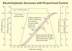
Shown is the input-output response of uncompensated and compensated servo systems.
System Tuning with Feed-Forward
Feed-forward tuning is done after the system is built and operational. Consider a servo axis with proportional control that has been tested, and with results shown in the illustration. The position-command profile is represented by plot A (red), the measured-output response by plot B, and the trapezoidal velocity-command profile by plot V. Mathematically, the position-command profile is the integral of the velocity command profile.
Note that the actual response lags behind the position command profile, a condition already identified as following error. The vertical separation of the two plots is essentially constant during the linear (constant-velocity) portions of the profile. Assume that the separation has been measured and found to be 0.6667 in. Note that this following error occurs with a velocity of 13.33 in./sec.
Here is the classic argument for and explanation of feed-forward: If the actual output lags the command by an intolerable amount, why not simply start the command a requisite amount earlier? After the natural servo loop lag, shouldn’t the actual response be very nearly where we want it? This is precisely what is done with feed-forward. Referring again to the illustration, the modified command profile, C, leads the desired position output by the amount of following error as measured. Thus, the actual response, A (blue), very closely agrees with the targeted command profile, also labeled A.
The only remaining question is how to modify the command profile. Because error must exist to generate velocity, we simply add a scaled portion of the velocity command profile to the original position command profile. That is:
XC,M = XC,O + KVFFVC
Where XC,M is the modified command profile
XC,O is the original, unmodified profile
VC is the velocity command profile, and
KVFF is the feed-forward scaling factor to offset the following error. It is found from:
KVFF = ∆XFE ÷ VSS
Where: ∆XFE is the measured following error, which was 0.6667 in. in the example, and
VSS is the constant speed plateau in the velocity command profile shown as 13.33 in./sec.
Feed-forward is relatively simple to implement at tuning time if the motion controller can maintain the original, unmodified profile plus the actual output response. An alternative is to use peripheral equipment to acquire such data. Lacking that, feed-forward — or any kind of tuning beyond simple proportional control — is nearly impossible to obtain. Because feed-forward parameters exist outside the servo loop, changing feed-forward parameters will not affect stability in most essentially linear systems.
When properly tuned, a feed-forward controller can eliminate following error during periods of constant velocity. Some residual following error will occur when the command profile calls for acceleration or deceleration. But accel/decel feed-forward compensation can be provided, too. Some motion controllers make provision for acceleration feed-forward. And even more sophisticated systems accommodate higher derivatives; each, in principle, removes a bit of the following error.
However, when derivatives of higher order than acceleration are used, the command profiles cannot be constructed with a velocity trapezoid, as was used in the illustration. Instead, they must use so-called “S-curve” velocity profiles. The rule is that the higher the order of derivative to be fed forward, the higher the order polynomial that must be used in the synthesis of the profile. If n represents the highest feed-forward derivative, then the nth derivative of the command profile must be finite.
Limitations to Feed-Forward
Of course, feed-forward is not a panacea. It cannot accommodate changes in the electrohydraulic system. For example, if actuator leakage increases, the feed-forward scaling factor that was found during leak-free setup tuning will be incorrect. Also, load changes render the feed-forward scaling factor incorrect. Because feed-forward compensation has no feedback, a controller cannot adjust to any changes in the electrohydraulic system servo loop.
On the other hand, feed-forward has excellent robustness to changes in the command profile. For example, feed-forward is vital in a flying cutoff system to prevent having to retune the controller every time a new in-feed rate must be accommodated.
For feed-forward to succeed, the valve and actuator must provide a linear velocity gain throughout the entire in-feed range. The above equations, incidentally, apply only if the servo valve has essentially linear metering characteristics. To accommodate any changes in the hydraulic system, integral control, which will be discussed in the next installment, must be implemented.